A model of a frequency distribution is an algebraic expression describing the relative frequency (height of the curve) for every possible score. The questions that sometimes come to the mind of the student is "What is the advantage of this level of abstraction? Why is all this necessary?" The answers to these questions may be found in the following.
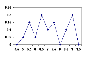
For example, suppose that the distribution of shoe sizes collected from a sample of fifteen individuals resulted in the following relative frequency polygon.
Because there are no individuals in the sample who wear size eight shoes, does that mean that the store owner should not stock the shelves with any size eight shoes? If a different sample was taken, would an individual who wore a size eight likely be included? Because it can reasonably be assumed that the reason no size eights were found in the sample was because of chance or sampling error, some method of ordering shoes other than directly from the sample distribution must be used.
In order to better deal with random fluctuations when collecting information from a sample, the statistician has the option of creating a model of the sample frequency distribution. This model is called by different names, including, probability model, theoretical probability distribution, probability density function (pdf), or simply population. A probability model attempts to capture the essential structure of the real world by asking what the world might look like if an infinite number of scores were obtained and each score was measured infinitely precisely. Nothing in the real world is exactly distributed as any given probability model. However, a probability model often describes the world well enough to be useful in making decisions.
If this were the case the proportion (.12) or percentage (12%) of size eight shoes could be computed by finding the relative area between the real limits for a size eight shoe (7.75 to 8.25). The relative area between scores on any probability model is called probability. In this case, the probability of a randomly selected woman wearing a size eight shoe would be .12. The concept of area under a curve will be covered in more detail in a later chapter.
The probability model attempts to capture the essential structure of the real world by asking what the world might look like if an infinite number of scores were obtained and each score was measured infinitely precisely. Nothing in the real world is exactly distributed as a probability model. However, a probability model often describes the world well enough to be useful in making decisions.
The statistician has at his or her disposal a number of probability models to describe the world. Different models are selected for practical or theoretical reasons. Some example of probability models follow.
The uniform distribution is shaped like a rectangle, where each score is equally likely. An example is presented below.
If the uniform distribution was used to model shoe size, it would mean that between the two extremes, each shoe size would be equally likely. If the store owner was ordering shoes, it would mean that an equal number of each shoe size would be ordered. In most cases this would be a very poor model of the real world, because at the end of the year a large number of large or small shoe sizes would remain on the shelves and the middle sizes would be sold out.
The uniform distribution is a useful model when the phenomena being modeled is relatively stable over a range of values. For example, the relative frequency of births on any day of the year in United States is relatively constant. In this case a uniform distribution might be an adequate, but not perfect, model
The negative exponential distribution is often used to model real world events which are relatively rare, such as the occurrence of earthquakes. The negative exponential distribution would be a good model of the relative frequency of lottery winnings. An overly optimistic distribution is presented below::
Not really a standard distribution, a triangular distribution could be created as follows:
It may be useful for describing some real world phenomena, but exactly what that would be is not known for sure. The statistician has the option of creating a distribution for a particular situation if mathematical equations can be found to describe the model. The statistician is not limited to only distributions that are widely used or that others have already discovered.
The normal curve is one of a large number of possible distributions. It is very important in the social sciences and will be described in detail in the next chapter. An example of a normal curve was presented earlier as a model of shoe size.
As described earlier, the statistician has the option of creating his or her own probability models. These models must be created using certain mathematical rules. These rules provide the properties of probability distributions.
The models that have been discussed up to this point assume continuous measurement. That is, every score on the continuum of scores is possible, or there are an infinite number of scores. In this case, no single score can have a relative frequency because if it did, the total area would necessarily be greater than one. For that reason probability is defined over a range of scores rather than a single score. Thus a shoe size of 8.00 would not have a specific probability associated with it, although the interval of shoe sizes between 7.75 and 8.25 would.